coding Archives - Perfect 3D Printing Filament

Coding for 3D Part 4: Rhino, Grasshopper and Weaverbird Setup

After doing research on how we are going to attack this series with our toolbox of resources, we are setting up our environment for exploration. Setting up the build environment is simple enough, but it is vital. Even with our build environment, there are specific subtle things we need to do for our purposes of creation. We will go through some of these items in this article while highlighting some other integral parts.

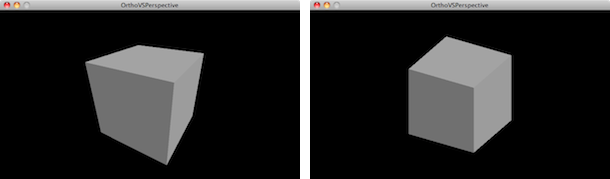
Firstly we need to download Rhino for our modeling purposes. To do so check out this link for a free 90 day trial version of Rhino. After going through the download instructions, we can now use Rhino. When I first opened Rhino, frankly I was intimidated. I have used various 3D modeling environments and software, but Rhino’s interface is a lot to handle. No disrespect to Rhino as a package as it is great, but it seems to have a steep learning curve. It has various plugins and tools ready for your disposal. Something important to remember is that having various tools is often not the best route when building anything. This is a methodology I take in terms of technical project building as well as physical product manufacturing. My goal with Rhino is to build parametric designs through coding, so I have a precise route to learning. This allows me to get to the meat of what I want to do quickly. I would not benefit from a large overview of Rhino at this point. A lot of what Rhino has tool wise does look intriguing, but we will stay focused when using it. Otherwise our curiosity may let us stray from our path to getting things done.

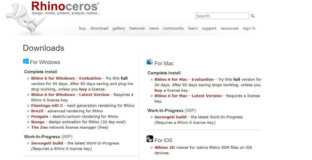
Download Window for Rhinoceros

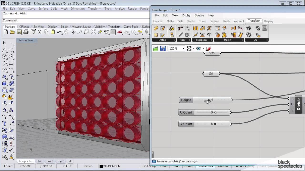
The biggest advantage of Rhino is the number of plugins available for it. These plugins are the essence of utility. We will focus on two plugins for Rhino in this series. The first plugin of interest to use is Grasshopper. Grasshopper is an algorithmic modeling plugin for Rhino. It uses a visual programming language vs. a typical text-based coding language. It also gives you the ability to reference geometrical objects from Rhino. The ability to create intriguing geometry quickly and with comparative ease is the main benefit of Grasshopper.

Grasshopper Build Environment

The second plugin of choice for us is Weaverbird. Weaverbird is a topology based modeler. It gives a designer the ability to make known subdivisions and transformation operators. This plugin allows us to automate subdivisions and reconstructing of shapes. It is a great plugin due to its ability to help in fabrication as well as rapid prototyping of ideas.

Weaverbird

Something I appreciate from Rhino is how extensive the program is from just looking at it briefly. Various software packages I have used are expansive, but Rhino seems to take things to a different level. The mind of an architect is very expansive, so their tool of choice needs to have various tools within its utility belt. I am excited to somewhat learn the mindset of an “architect” through operating in this program.

For the next installment of this series, we will try to make a simple 2D parametric design that can be extruded into 3D form. I realize the importance of 2D drawing and going to the 3D level as it makes product creation much easier. It flows better and it makes the ability to iterate more intuitive. So look out for that in our next article.

The post Coding for 3D Part 4: Rhino, Grasshopper and Weaverbird Setup appeared first on 3DPrint.com | The Voice of 3D Printing / Additive Manufacturing.

What is Metrology Part 22 – 3D Translation and Rotation

3D Translation

3D translation and rotation is vital within a 3D environment. We have discussed the importance of this within metrology previously in CMM systems. Interfacing the physical world and digital world requires precise measurement coordinates. Within 3D environments, movement is vital. In particular, movement is our focus today. We will talk about how example code within Processing can help us interface the digital world and physical realm. How does one simulate the real world within a virtual space? VR and 3D build environments are critical. So what are the basics needed for measurement and calculating space in a digital field? Metrology systems and laser scanning help. Tracking movement in terms of translation within a coordinate system is vital. So how could we learn about the basics of all of this? Let’s look into Processing as our main digital coding tool. How does Processing compute translational movement? If one wants to understand coding in a 3D environment, it is highly recommended that you understand object oriented program. We will not do a deep dive into this today, but a lot of the operations we are doing are object oriented. The following code is how I will demonstrate movement within Processing:

size(640,360,P3D);

background(0);

lights();

pushMatrix();

translate(130, height/2, 0);

rotateY(1.25);

rotateX(-0.4);

noStroke();

box(100);

popMatrix();

pushMatrix();

translate(500, height*0.35, -200);

noFill();

stroke(255);

sphere(280);

popMatrix();

Processing Example Code

Let’s take a look at this line by line. The first line is dedicated to building the 3D environment. The background of this window is denoted by the color value 0 which corresponds to black. The lights() function allows us to use ambient light, directional light, and specular values within our environment. In this case we are using the default light structure. pushMatrix(), we have discussed before as a function that allows us to set our original matrix of data that will be manipulated later. Our manipulation will come in the form of translational and rotational forces implemented. translate(130, height/2, 0) manipulation in question. The rotateY() function is used to move the window towards a particular angle based on units from the Y-axis of our viewport. The rotateX() function is similar except it is rotating within the X-axis. noStroke() allows us to be free from bordered 3D image renderings. box(100) allows us to create a 3D box with a float dimension of 100 in the x-dimension. popMatrix() ends the manipulation of the original data set. We then are able to start a new data manipulation through translation with pushMatrix(). This time, we have used the following command to apply a translation: translate(500, height*0.35, -200). Instead of a box though, we created a sphere for rotation.

Planar Rotation

We have focused a lot on coding basics within this metrology series as a whole. Being able to have standardized measuring devices within our metrology equipment is key. Without such, we would lack tangibility. If a 3D environment cannot be built with a computer, there is no way to interpret the data from a 3D world that we interact with. Being able to set a coordinate based on the world around us is still a difficult task though. So how can we do this? It makes us question how most of the devices we use in metrology are able to accurately set values of measurements based on the real world. These set of questions are things I would further like to explore.

The post What is Metrology Part 22 – 3D Translation and Rotation appeared first on 3DPrint.com | The Voice of 3D Printing / Additive Manufacturing.

What is Metrology Part 21 – Getting Started with Processing

3D Environment Simulation in Processing

In the previous article, I showed the awesome coding framework of Processing. It is fun and interactive for anyone new to code. It makes learning a simple breeze, and it lines up a lot with the topics we have covered within this series thus far. These topics include image processing, 3D image rendering, 3D scanning, pixelation, image restoration, and a slew of other applications. With this article, I will show you how to get started with this program.

To get started, one should visit Processing and their website. From there, you can go to their downloads page and find the corresponding installation package that is right for your system. The package for Processing will be found in a zip file in your downloads section once it is unpacked from the website. Within this download package you will click through it to find an icon that says processing. Once you click this your computer will prompt you to extract the file into a different location. After this you may now use Processing.

Processing Sketchbook

Once you open Processing you will notice the sketchbook and developing environment. That is where all of the code will be run and executed. In order to code within this environment, one needs to understand how to manipulate movement and vision within the 2D realm first before moving to 3D. I think having a solid foundation within 2D leads to better 3D thinking because geometry naturally flows this way. Processing is object oriented and it utilizes rotational and translational commands to make interesting visuals. The majority of commands used in 2D will be applicable to 3D. Processing fortunately has a 2D transformation tutorial online that is a great starting point for explaining the capabilities. Below is a snippet of code that is from the processing site and it has comments on what these lines mean.

void setup(){

  size(200,200); //size of the window

  background(255); //color value of the background

  noStroke(); //disables the border drawing of the stroke

  //draw the original position in gray

  fill(192); //Sets the color used to fill shapes.

  rect(20, 20, 40, 40); //draws the rectangle with these dimensions  

  //draw a translucent blue rectangle by translating the grid

  fill(0, 0, 255, 128); //fills a rectangle with the blue color

  pushMatrix(); // Pushes the current transformation matrix onto the matrix stack.

  translate(60, 80); //translates the original rectangle 60 units right and 80 units down

  rect(20, 20, 40, 40); //draws the location of the translated data of the original matrix

  popMatrix(); //  Pops the current transformation matrix off the matrix stack.

}

To initialize a build environment in Processing, one needs to setup the environment. Setup calls a function for a viewport to see the digital code. The window size is denoted as well as the background color. The noStroke() function disables Processing and its automatic border drawing for images.

Executed Script in Processing

Then a fill function is used to color any shape after this definition to be this color. To set the dimensions of our box, we used the rect() function. Then we wanted to create a new blue rectangle so we applied the fill function again but with different values. After this we want to apply translations to the original matrix data we had for the rectangle in terms of location. The pushMatrix() command essentially opens up a loop of interaction within our code to allow us to independently control objects within our environment. Then we are able to apply the translate function to our original matrix data. In this case we translated the data to the right 60 units and down 80 units. Then we ended this cycle by applying the command popMatrix().

3D Wireframe Processing

Whenever one wants to code, it is good practice to know what every command or function within your code means. Without knowledge of this, you are going to become a copy and paste coder who does not understand the nuances within their own code. It also will take you a bit more time to go through programming tutorials when you stop to learn exactly what everything means, but at a certain point you will gain a greater overall scope of the tools you have at your disposal. With this basic code example, we can expand our skills and apply this in 3D. In the next article, I will show how to do so.

The post What is Metrology Part 21 – Getting Started with Processing appeared first on 3DPrint.com | The Voice of 3D Printing / Additive Manufacturing.

What is Metrology Part 20 – Processing

Processing

Hey everyone! So this series thus far has been a bunch of fun, and it gets more exciting with what we are doing today. Today I’ll be taking us through a basic tutorial in coding through the framework of the Processing API. I have had experience with this programming language and I believe it is an interesting medium for visualizations of various sorts. It can do awesome generative computerized art, and it can be the source of interesting projects when data and 3D environments are fused. I’ll give an informational overview of the platform as it pertains to 3D manipulation.

Processing is an interesting platform as it is a software sketchbook in a sense. It is a language used for coding and applying it specifically to the visual arts. Processing has done a lot of promotion for software literacy within the visual arts field. It has also done similar promotion for visual literacy within the technology sector. They have built a large global community of students, artists, researchers, and hobbyists who use the platform for educational and prototyping purposes.

Processing Tutorials

I personally started messing with Processing when I was in college. I had some skills in Python mostly through my physics courses, but I was working at my Center of Digital Media within my university. Being around digital media and artistic individuals got me curious as to see the combination of technical fields as well as the arts. When I was learning to code a bit more, I found the Processing platform and a large amount of YouTube tutorials.

Generative Processing Art

Something of interest to me with the platform is that it is a simple interface. It also is not as intimidating of an environment compared to other development spaces. For someone who is interested in things such as image processing, it is the ideal platform to learn quickly. Combining the arts and technology seems disparate for a lot of people. These two fields however are extremely similar and they should not live in vacuums away from each other.

Another great thing about Processing is the large portfolio of onsite tutorials that explain the basics to someone who has no experience with the platform. They did a great job of explaining what every command does within their environment. When learning to code, it is more of a learn as you go approach. When one needs a function, they will have to research online for the meaning of this function and how to execute it. Processing did a good job of centralizing their information through their website and online forum communities.

P3D Mode in Processing

Processing’s power lies within its five render modes. These render modes are the default renderer, P2D, P3D, PDF, and SVG. The default renderer is the backbone of a lot of the programs done by Processing users. It is used for 2D drawing. The usage rates vary based on whether the other renders lack the definition of the size() parameter. The P2D renderer is an alternative to the default renderer for 2D images. The difference between these renderers is that P2D has a quicker runtime, but it sacrifices some visual quality for speed. The P3D renderer is used for drawing in three dimensional space. The PDF renderer is used for writing PDF files from Processing. The files can be scaled to various sizes and output with high resolutions. This renderer can also flatten 3D data into a 2D vector file as well. The SVG renderer does similar tasks as the PDF renderer, but the file format is an SVG. A lot of the renderer power for 3D imaging comes from utilizing the software of OpenGL that is supported on multiple GPUs to help speed up the drawing process.

With this overview, I hope I have intrigued people for a couple of coding projects I will try to show off within the series.

The post What is Metrology Part 20 – Processing appeared first on 3DPrint.com | The Voice of 3D Printing / Additive Manufacturing.

What is Metrology Part 16: Introductory Coding

Anaconda

Today we will be looking into the basics of image processing and coding within Python. We will start with 2D images and learn some elementary skills in terms of setup and coding with image processing. With all of the research being done in this metrology series, it will be fun to do some interactive and project-oriented learning that focuses our attention to the different subject matter we have touched so far. Be prepared to deep dive a bit more with me today.

The first step in coding is choosing and setting up one’s developing environment. This choice is done through knowledge of what language you are using, as well as personal preference. I myself have basic scripting skills within Python. My first inclination for coding is the Python language. This limits the scope of development tools that are available to me. I also am coding with the intent of doing image processing work. This dictates my workflow and environment.

Command Line Example

I decided to develop with the Anaconda environment for Python. The steps for downloading and running Anaconda can be a bit confusing if you do not have previous experience with a command line. A command line is the space to the right of the command prompt on an all-text display mode on a computer monitor (usually a CRT or LCD panel) in which a user enters commands and data. Commands are generally issued by typing them in at the command line and then pressing the ENTER key, which passes them to the shell. For someone completely new to coding though, there are various tutorials and online resources that are instruction based. I will layout the process that I used to get my development environment setup:

Download the Anaconda package through here.

When the installer gives you the option to add this to your environment path be sure to do so. It is important for later interactions with your computer’s command line.

Use the following conda command in your command line when Anaconda is installed:

conda install jupyter

Once this command is entered, your computer will unzip the jupyter notebook package from the web. A jupyter notebook is where one can place their Python code. It can also be executed and tested within this environment. It is an awesome tool for developing.

Use the following conda command in your command line after completing the previous installation:

conda install pillow

Once this command is entered, your computer will unzip the pillow package from the web. The pillow package is a great package for Python because it imports functions that are specific to image processing techniques. Once those installations are done, open a new command line and type in the following command:

jupyter notebook

Jupyter First Glance

This will open up a jupyter notebook environment within one of your browser tabs automatically. From there we are now able to start coding and have some fun. There is a button on the upper right hand corner that says new. Click this and press Python 3 for the ability to make a file for developing. The initial popup window should correspond to how your desktop environment is setup in terms of files.

Now that we have all of this setup, please take a look at this online tutorial here. In this tutorial it is one should copy and type all of the text that appears within the code posted. Without exact formatting, various errors may pop up as you run your program. This is the more challenging part of programming. Being able to spot errors and bugs when we are creating projects is the essence of a succinct programmer. There will also be various items, words, and functions that seem complex. It is important for one to learn everything that seems foreign to them if they want to become an excellent programmer.

Antialiasing Example

I myself had no real understanding of the word antialiasing. It is something I have seen before in my camera settings of a DSLR I use, and I have seen it within programs such as Photoshop, but I really did not understand what it was. Once I saw it in the context of code, I really had to understand what it meant. In the particular code snippet I copied from the tutorial, the goal was to create images that were at a certain size and shape. In order for images to be compressed, antialiasing is an important factor. Antialiasing is a technique used to add greater realism to a digital image by smoothing jagged edges on curved lines and diagonals. This is a computer graphics technique that allows for sharper resolutions for a photo based on precise geometry. Some of the “imperfections” of an image may be distorted or destroyed due to this. I am certain that in order to do processing such as photogrammetry and image stitching, a computer would have to have exact geometries that can be added together to form a 3D image. This causes the 3D image to have less precision overall in terms of actual dimensions. I wonder what is the margin of error for a 3D image when photogrammetry techniques are accounting for antialiasing.

Lastly, I learned about an alpha channel. Alpha channels are color components that represent the degree of transparency (or opacity) of a color (i.e., the red, green and blue channels). They are used to determine how a pixel is rendered when blended with another. It now begs the question of how precise are metrology and laser scanning devices in terms of picking up color. These are follow up questions I will be researching more in depth.

Overall, this is the first step into the world of image processing. I am excited to continue research as well as build out fun projects that will show off this field a bit more.

The post What is Metrology Part 16: Introductory Coding appeared first on 3DPrint.com | The Voice of 3D Printing / Additive Manufacturing.